A Poisson Maximum Likelihood Model for prediction and evaluation of MLB teams and pitchers

This article was originally published in 2016 at jackoliverwerner.wordpress.com.

Introduction

Sports are all about matchups: two teams battling it out on the court, rink, or field until one side emerges the winner. Head-to-head matchups are an especially prominent component of baseball. The game is an overarching matchup of one team against another, but it contains smaller competitions: a pitcher and a catcher trying to outscheme an opposing hitter, a second baseman playing cat-and-mouse to hold a runner close to the bag, or a starting pitcher with a scissors trying to get out of wearing throwback jerseys.

So it only makes sense that we use matchups as comparisons to evaluate teams and players. When we see the local nine win a game, it’s a good sign. But how good? It depends on their competition. If I head over to Target Field and watch a Twins victory, my evaluation of their performance will differ if they’re facing the Gophers in an exhibition versus if they beat the AL pennant-winning Indians (and if it was a game Corey Kluber started, all the better). In short, we know the Twins are good if they beat good teams.

But this just shifts the question: how do we know if the Twins’ opponents are any good? Well, we can evaluate the Twins’ opponents’ opponents to see who they were able to beat. But this leads to evaluating their opponents, and on and on. Clearly, this gets complicated. (Especially considering that the Twins’ opponents’ opponents include the Twins themselves!) The results of an MLB season are a web of interrelated, intertwined information. To make sense of it all, I developed what I call a Poisson Maximum Likelihood (PML) model to score teams and pitchers. I was inspired by the Bradley-Terry Model, so let’s start there.

The Bradley-Terry Model

The Bradley-Terry Model attempts to predict the outcome of any comparison between two elements of a group (like teams in a league). Each team is assigned a score based on their relative strength—the higher the score, the better the team. Given two teams with scores $a$ and $b$ , the probability of the first team winning is $\frac{a}{a + b}$ .

But how are these scores calculated? The Bradley-Terry Model takes in the results of some games that have been played, and it finds the set of scores that would give the best possible predictions for these games. ¹ This process is called maximum likelihood estimation.

The Bradley-Terry Model is appealing in its simplicity and elegance. It’s likely too simple to apply to baseball, though, for a couple of reasons. Mainly, it doesn’t account for starting pitching, which makes a big difference. For example, in 2016, the White Sox allowed an average of 6.0 runs in the 22 games where James Shields was the starter, but only 3.1 in the 32 games started by Jose Quintana. Additionally, the Bradley-Terry model doesn’t account for margin of victory, or account separately for offense and defense. I created a model which includes these factors, while retaining the maximum likelihood estimation—and hopefully the theoretical elegance—of the Bradley-Terry Model.

The Poisson Maximum Likelihood Model

In my proposed model, each team and each starting pitcher is assigned a score. The team score represents offensive capability, while the pitcher score represents overall defensive capability when that pitcher starts a game. The distribution of runs scored by a given team in a game started by a given pitcher is modeled as a Poisson distribution, with $\lambda$ equal to the team’s score multiplied by the pitcher’s score. For each game, then, this model gives two Poisson distributions to model the runs scored by each team. These can be used to calculate the probability of each team winning (optionally with a home-team adjustment). Similarly to Bradley-Terry, the team and pitcher scores are assigned such that they best predict runs scored for a set of games already played. See the appendix at the end for a more detailed explanation of the methodology.

An advantage of this model is its simplicity. Assigning one score per team and pitcher means the model is interpretable. In this formulation, a higher team score denotes a team with a relatively better offense. A lower pitcher score is better, but its interpretation is a little bit more complicated; pitcher scores are tied to pitcher ability, but also to their team’s bullpen and defensive ability. In theory, this means that this model accounts for all phases of the game—offense, starting pitching, bullpen, defense—in a way that is more nuanced than a Bradley-Terry model, yet still relatively simple.

This simplicity does lead to limitations. Predictions for pitchers traded mid-season may be less accurate, as the model is built using games where they were supported by different bullpens and defenses. Additionally, there are other factors that influence a baseball game’s outcome, such as platoon splits, park effects, and home field advantage. (I apply a rough correction for the last of those after the fact in my predictions, but it’s not accounted for in the fitting of the model). Finally, the model uses basic metrics (team runs scored, team runs allowed), which could potentially be noisier than other statistics which are more related to true talent (FIP, wOBA).

Model Results

To get a feel for model results, let’s take a look at 2016. Here are the team (offense) scores:

Team	Score
BOS	2.57
COL	2.39
SEA	2.28
DET	2.28
CHC	2.28
CLE	2.27
TEX	2.22
STL	2.22
BAL	2.22
TOR	2.22
ARI	2.20
WSN	2.15
MIN	2.13
PIT	2.13
HOU	2.11
LAA	2.10
CIN	2.08
LAD	2.07
SFG	2.06
NYY	2.06
TBR	2.03
CHW	2.02
KCR	2.01
SDP	1.99
NYM	1.93
OAK	1.93
ATL	1.93
MIA	1.92
MIL	1.92
PHI	1.76

And here are the top 10 pitcher scores (keep in mind that these represent a pitcher as well as his bullpen and defense).

Pitcher	Score
Clayton Kershaw	0.81
Rich Hill	1.27
Drew Pomeranz	1.36
Jose Quintana	1.41
Jon Lester	1.42
Johnny Cueto	1.42
Jose Fernandez	1.46
Kyle Hendricks	1.47
Kevin Gausman	1.48
Chris Tillman	1.50

Interpretation would go something like this: if Clayton Kershaw started a game against the Red Sox, we would expect Boston to score $2.57 \cdot 0.81 = 2.08$ runs, on average.

There are no huge surprises on either list. We already knew that Clayton Kershaw is otherworldly, and that the Red Sox had a formidable lineup. But lack of surprise is a good sign! If Shelby Miller had topped the list, it probably wouldn’t mean that the model has discovered some hidden value in his 6.15 ERA and 4.87 FIP. It probably would mean that something is off about the model.

Possibly the biggest surprise is Colorado claiming the number two offensive spot. Though this isn’t in line with their offensive reputation, their high score can be explained by Coors Field. This ranking is less a complete head-scratcher, and more a sign to be wary that park effects could skew results.

Model Predictions

For every season from 1998 to 2016, I used this Poisson Maximum Likelihood (PML) model to create scores based on the regular season, then used these results to predict all postseason matchups. For the sake of a benchmark, I compared it to a simple model using each team’s regular season winning percentage.² I want to see not only whether this model does better than random guessing, but also whether it does better than naive guessing. (And if I can get predictions that are just as good with less work, that’d be nice to know!) I also created versions of both my model and the simple model which account for home-field advantage.³ This gave four models total. I evaluated each model on accuracy (how often did the team with a greater chance to win actually win?) and Brier score (a more complete measure of predictive accuracy, where lower is better).

	PML Model	PML Model with Home-Field Adjustment	Simple Model	Simple Model with Home-Field Adjustment
Accuracy	52.8%	55.1%	50.9%	55.0%
Brier Score	0.257	0.255	0.249	0.247

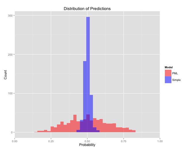
Each model (the adjusted and un-adjusted) did better than its simple counterpart, but only by a tiny amount. The Brier scores are worse for the PML models than for the simple ones. It seems like this is a result of a calibration issue. The PML models give more extreme score predictions, while the simple model hovers around 50/50 (seen below). It seems likely that the PML model is overconfident, meaning that the model gives predictions with more certainty than it should. Perhaps this is because a team’s runs scored in a game isn’t well-modeled with a Poisson distribution, or perhaps there’s another explanation.

rplot

Conclusions

The strength of this method seems to be scoring and ranking rather than prediction. There’s little evidence that the PML in its current form outperforms even a simple alternative model. In the future, it would be worth re-evaluating the use of a Poisson distribution in modeling runs scored, and possibly looking into incorporating park effects. Nonetheless, this is an interesting exercise. I believe there’s value in a maximum likelihood-based team and player evaluation metric because it directly accounts for the interconnected web of matchups that is an MLB season.

Code and data for this project can be found on my Github page.

Footnotes

More formally, the model finds the set of scores which maximizes the likelihood of a group of actual results given the predicted probabilities. ^{^}
Given a team’s regular season winning percentage $WP$ and their opponent’s winning percentage $oWP$ , I calculated that team’s probability of winning as $\frac{WP}{WP + oWP}$ . ^{^}
An interesting note: the simple, home-field adjusted model picked the home team to win all but 14 out of 631 games. Since the home team has won roughly 54% of all playoff games, this provides another useful benchmark. Hopefully the PML model does better than just picking the home team! ^{^}

Appendix

An explanation of the gory mathematical detail. In this model, each team and starting pitcher is given a score. Pitchers with small numbers of starts would have scores which are too unstable, so they are lumped together into an “other” category. Fitting is done as if the “other” category were all one pitcher. Roughly, this can be thought of as a “replacement-level” starter, as pitchers with fewer starts tend to be more mediocre. I use a threshhold of 15 starts, as it seemed to produce stable scores while allowing as many unique pitchers as possible.

To determine how well a set of scores fits some actual results, we must calculate a likelihood. Given a set of scores, the model first calculates the likelihood of each matchup (offense vs. starting pitcher) in each game. For each of these matchups, a $\lambda$ is given by the product of the scores of the offense and the opposing starting pitcher. The likelihood for each side is then calculated based on the actual number of runs scored according to a Poisson distribution with the given lambda. The product of all these likelihoods is the overall likelihood.

More formally: given $n$ teams and $m$ starting pitchers, where the most runs scored by a team in a game is given by $x$ , let $R_{i}$ and $RA_{j}$ be the scores for team $i$ and pitcher $j$ , respectively. Also let $s_{ijr}$ be the number of times team $i$ has scored $r$ runs in a game started by $j$ . Then the likelihood function for the Poisson Maximum Likelihood model is given by:

$\displaystyle \prod_{i=1}^{n} \prod_{j=1}^{m} \prod_{r=0}^{x} \left(\frac{(R_{i}RA_{j})^{r}e^{-R_{i}RA_{j}}}{r!}\right)^{s_{ijr}}$

And the log-likelihood function is given by:

$\displaystyle \sum_{i=1}^{n} \sum_{j=1}^{m} \sum_{r=0}^{x} s_{ijr}r\log(R_{i}RA_{j}) - s_{ijr}R_{i}RA_{j} - s_{ijr}\log(r!)$

The last term is independent of the scores, so it can be eliminated. I also add a term to apply the constraint that the mean of pitcher scores, weighted by starts, is equal to the mean of team scores, weighted by games. (Without this constraint, there are an infinite number of optimal solutions.) Let $s_{i}$ denote the number of games played by team $i$ and $s_{j}$ denote the number of games started by pitcher $j$ . This gives a new score function of:

$\displaystyle \sum_{i=1}^{n} \sum_{j=1}^{m} \sum_{r=0}^{x} \left[s_{ijr}r\log(R_{i}RA_{j}) - s_{ijr}R_{i}RA_{j}\right] + a\cdot\left(\frac{\sum_{i=1}^{n} R_{i}s_{i}}{\sum_{i=1}^{n} s_{i}} - \frac{\sum_{j=1}^{m} RA_{j}s_{j}}{\sum_{j=1}^{m} s_{j}} \right)^2$

(Note that $a$ is a constant used to adjust the relative importance of likelihood term to difference-in-means term). To find the values of the scores, I used this score function in a gradient ascent algorithm. To calculate the gradient, I had to find the partial derivative of the scoring function with respect to each individual score. For team scores, this is given by:

$\displaystyle \frac{d}{dR_{i}} = \sum_{j=1}^{m} \sum_{r=0}^{x} \left[s_{ijr}\left(\frac{r}{R_{i}} - {RA_{j}}\right)\right] + 2a\frac{s_{i}}{\sum_{i=1}^{n} s_{i}}\left(\frac{\sum_{i=1}^{n} R_{i}s_{i}}{\sum_{i=1}^{n} s_{i}} - \frac{\sum_{j=1}^{m} RA_{j}s_{j}}{\sum_{j=1}^{m} s_{j}} \right)$

For pitcher scores, this is given by:

$\displaystyle \frac{d}{dRA_{j}} = \sum_{i=1}^{n} \sum_{r=0}^{x} \left[s_{ijr}\left(\frac{r}{RA_{j}} - {R_{i}}\right)\right] - 2a\frac{s_{j}}{\sum_{j=1}^{m} s_{j}}\left(\frac{\sum_{i=1}^{n} R_{i}s_{i}}{\sum_{i=1}^{n} s_{i}} - \frac{\sum_{j=1}^{m} RA_{j}s_{j}}{\sum_{j=1}^{m} s_{j}} \right)$

Once the algorithm converges on a maximum, we have our scores. From these, we can predict runs scored in a game using a Poisson distribution with $\lambda = R_{i}RA_{j}$ . This value can also be adjusted for home field advantage. Home teams tend to win MLB games 54% of the time, which equates to a 17% increase in odds (and a 17% decrease in odds for the away team). We adjust the odds for the home team by 1.17. In terms of probabilities, given unadjusted probability $p$ , the adjusted probability $p'$ is equal to:

$\displaystyle p' = \frac{1.17p}{1-0.17p}$

Model 284

Analyzing sports through math and models