Similarity Score Methodology

Introduction

“Buddy Hield is the next Stephen Curry”
“Brandon Ingram is a poor man’s Kevin Durant”
“Andrew Wiggins’ upside is Carmelo Anthony, but his floor is James Posey”

So often when we talk about NBA players, we do it through comparisons to other players, and with good reason—comparisons are a good way to quickly convey lots of information about a player. For example, if I tell you that a player had a Box Plus/Minus of 7.8 last season, you might get a vague idea of how good he is. If I then tell you that player had 19.5 points per game, you might have a slightly better idea, but it’s still far from the full picture. But if I claim that this player is the next Chris Paul, it immediately brings to mind an idea of not only how good he is, but also his strengths, weaknesses, and overall playing style. Maybe your mind also queues up a mental highlight reel of Chris Paul-like plays, for good measure. Comparisons quickly give a complete picture of a player which would otherwise require taking the time to slowly digest each number in his stat line.

Also, they’re lots of fun!

We’ve created our own set of similarity scores to make comparisons using math for the purpose of prospecting players coming out of college. Our goal is to produce a useful complement to our PNSP model. Where our PNSP model answers the question, “How valuable will this player be?”, our similarity scores aim to answer the question, “Who will this player be like?”

For a glimpse of some player comparisons, you can check out Similarity Scores for 2016 NBA Draftees, here.

Data

Our dataset consists of players who entered the league between 1997-2016. International players, high school players, and players with incomplete college statistics are excluded from the data. Since data record-keeping has become more reliable in recent years, our data contains more players from more recent draft classes. This is only an issue in that it limits the size of our training data; skewing more recent may help to better capture current trends in the NBA.

Methodology

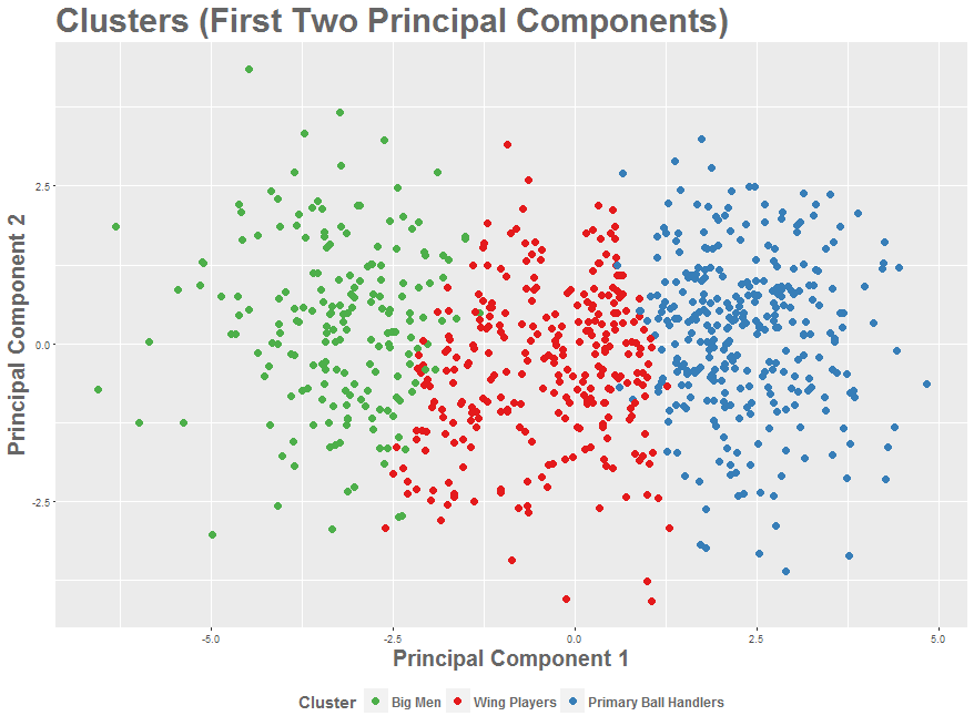
We started by dividing our players by position, in order to create similarity score calculations differently for different types of players. After all, the things you care about when deciding whether two big men are similar is very different than when you’re comparing two point guards. Rather than doing this grouping using our intuition, we used k-means clustering to form groups based on box-score statistics. This technique allowed the data to determine how the players should be grouped, potentially identifying players who fit best in a group other than their nominal position. Ultimately, though, the three clusters we created ended up corresponding intuitively to three player archetypes: primary ball handler, wing player, and big man. Below is a chart showing these clusters, visualized with Principal Component Analysis. PCA is a statistical procedure with many interesting uses. Here, it’s just used as a visualization tool, so the important thing to know is that combines our many original variables into two new ones, which allow us to get a two-dimensional picture of as much of our data as possible. To get a player’s coordinates to find him on this chart, use our table below.

Player	Clustered Group	PC1	PC2
A.J. Bramlett	Big	-3.07	0.79
A.J. Guyton	Primary Ball Handler	2.75	0.26
A.J. Hammons	Big	-4.19	-1.29
A.J. Price	Primary Ball Handler	2.45	0.78
Aaron Brooks	Primary Ball Handler	3.57	0.03
Aaron Gordon	Wing	-0.94	3.16
Aaron Gray	Big	-4.48	0.54
Aaron Harrison	Primary Ball Handler	3	1.2
Aaron White	Wing	-0.14	-1.84
Abdel Nader	Wing	0.58	0.84
Acie Law	Primary Ball Handler	2.13	-0.98
Adam Morrison	Wing	0.33	-2.61
Adonal Foyle	Big	-5.99	-1.25
Adreian Payne	Wing	-0.74	-0.95
Al Horford	Big	-3.13	0.23
Al Thornton	Wing	0.04	-1.32
Al-Farouq Aminu	Wing	-1.72	0.08
Alan Anderson	Wing	0.13	-1.67
Alando Tucker	Wing	0.17	-0.94
Alec Brown	Wing	-1.21	-0.91
Alec Burks	Wing	0.42	-1.94
Alex Acker	Primary Ball Handler	1.7	-0.4
Alex Len	Big	-3.18	0.36
Alex Oriakhi	Big	-3.91	-0.84
Alexander Johnson	Wing	-1.67	-1.25
Allen Crabbe	Primary Ball Handler	1.09	0.14
Alton Ford	Wing	-1.33	0.79
Alvin Jones	Big	-3.86	0.55
Alvin Williams	Primary Ball Handler	1.95	0.3
Andre Drummond	Big	-4.48	4.36
Andre Emmett	Wing	-0.12	-0.85
Andre Iguodala	Primary Ball Handler	0.89	0.52
Andre Miller	Primary Ball Handler	1.41	-0.23
Andre Roberson	Wing	-0.71	2.13
Andrew Bogut	Big	-2.94	-0.89
Andrew Goudelock	Primary Ball Handler	2.52	-1.58
Andrew Harrison	Primary Ball Handler	2.78	0.89
Andrew Nicholson	Wing	-2.31	-2.19
Andrew Wiggins	Wing	0.53	0.48
Andy Rautins	Primary Ball Handler	3.27	0.7
Anthony Bennett	Wing	-1.77	-0.43
Anthony Brown	Primary Ball Handler	1.84	0.01
Anthony Davis	Big	-4.06	0.72
Anthony Johnson	Primary Ball Handler	2.05	-1.48
Anthony Morrow	Primary Ball Handler	2.35	0.33
Anthony Parker	Primary Ball Handler	1.15	-0.75
Anthony Randolph	Big	-2	0.97
Antoine Wright	Wing	0.83	0.01
Antonio Burks	Primary Ball Handler	2.73	1.32
Antonio Daniels	Primary Ball Handler	2.14	-1.92
Archie Goodwin	Wing	0.58	1.08
Armon Johnson	Primary Ball Handler	1.04	0.74
Arnett Moultrie	Wing	-1.02	-0.84
Arron Afflalo	Primary Ball Handler	1.76	0.54
Arsalan Kazemi	Big	-1.83	0.36
Austin Croshere	Wing	0.44	-1.49
Austin Daye	Wing	-1.3	0.26
Austin Rivers	Primary Ball Handler	1.82	1.5
Avery Bradley	Primary Ball Handler	1.74	3.24
Baron Davis	Primary Ball Handler	1.52	1.13
Ben Bentil	Wing	-0.93	-1.05
Ben Gordon	Primary Ball Handler	3.14	0.15
Ben McLemore	Primary Ball Handler	2.21	0.49
Ben Simmons	Wing	-0.65	-0.27
Bernard James	Big	-3.62	2.16
Bernard Robinson	Primary Ball Handler	1.14	0.4
Blake Griffin	Big	-2.89	-0.98
Bobby Jackson	Primary Ball Handler	2.13	0.57
Bobby Jones	Wing	0.71	0.01
Bobby Portis	Wing	-2	-0.66
Bobby Simmons	Wing	0.54	-0.5
Bracey Wright	Primary Ball Handler	1.56	0.07
Bradley Beal	Primary Ball Handler	1.39	0.98
Brandan Wright	Big	-3.44	1.77
Branden Dawson	Big	-2.44	2.48
Brandon Armstrong	Primary Ball Handler	2.06	-1
Brandon Bass	Wing	-1.83	-1.04
Brandon Hunter	Wing	-2.18	-1.52
Brandon Ingram	Wing	0.5	1.76
Brandon Knight	Primary Ball Handler	2.78	1.23
Brandon Roy	Primary Ball Handler	1.4	-1.72
Brandon Rush	Primary Ball Handler	1.59	1.09
Brendan Haywood	Big	-5.1	1.28
Brevin Knight	Primary Ball Handler	4.83	-0.63
Brian Cardinal	Wing	1	-0.31
Brian Cook	Wing	-1.39	-2.49
Brian Scalabrine	Wing	-0.16	-0.09
Brice Johnson	Big	-2.86	-0.74
Brook Lopez	Big	-3.13	-1.19
Bubba Wells	Wing	-0.12	-4.04
Buddy Hield	Primary Ball Handler	2.25	-1.19
C.J. McCollum	Primary Ball Handler	2.53	-3.32
C.J. Wilcox	Primary Ball Handler	2.19	-0.39
Cady Lalanne	Big	-3.43	0.03
Cal Bowdler	Big	-2.68	-1.66
Calvin Booth	Big	-3.29	0.03
Cameron Bairstow	Wing	-1.97	-2.48
Cameron Payne	Primary Ball Handler	2.78	-1.07
Caris LeVert	Primary Ball Handler	1.9	-0.59
Carl Landry	Wing	-1.66	-1.57
Carlos Boozer	Big	-3.85	-1.94
Carmelo Anthony	Wing	-0.52	0.16
Caron Butler	Wing	0.11	-0.6
Carrick Felix	Wing	0.66	1.08
Casey Jacobsen	Primary Ball Handler	1.39	-0.97
Cedric Henderson	Wing	0.05	0.35
Cedric Simmons	Big	-2.65	0.55
Chandler Parsons	Wing	0.16	1.76
Channing Frye	Big	-2.4	-0.9
Charles Jenkins	Primary Ball Handler	2.14	-2.08
Charles Smith	Primary Ball Handler	1.56	-0.66
Charlie Villanueva	Wing	-2.09	-0.34
Chase Budinger	Primary Ball Handler	1.61	0.17
Chauncey Billups	Primary Ball Handler	3.45	-1.05
Chinanu Onuaku	Big	-3.8	2.05
Chris Bosh	Wing	-1.78	-0.12
Chris Crawford	Wing	0.12	-0.81
Chris Douglas-Roberts	Wing	0.41	-0.93
Chris Duhon	Primary Ball Handler	2.35	1.89
Chris Herren	Primary Ball Handler	3.99	0.91
Chris Jefferies	Wing	0.54	0.3
Chris Kaman	Big	-4.98	-3.02
Chris McCullough	Big	-1.89	2.71
Chris Mihm	Big	-3.39	-1.26
Chris Owens	Big	-2.19	-0.62
Chris Paul	Primary Ball Handler	4.1	0.32
Chris Porter	Wing	-0.39	0.42
Chris Richard	Big	-3.03	0.89
Chris Singleton	Wing	0.36	0.77
Chris Taft	Big	-3.98	0.82
Chris Wilcox	Big	-2.71	1.55
Christian Wood	Big	-3.03	-0.64
Cleanthony Early	Wing	0.96	-1.42
Cody Zeller	Wing	-1.67	-0.62
Cole Aldrich	Big	-4.61	0.46
Colton Iverson	Big	-3.47	-0.32
Corey Brewer	Primary Ball Handler	1.6	0.39
Corey Brewer1	Primary Ball Handler	1.6	0.39
Corey Maggette	Wing	-0.28	-0.23
Corsley Edwards	Big	-2.42	-2.74
Cory Jefferson	Wing	-1.19	0.27
Cory Joseph	Primary Ball Handler	2.15	2.43
Courtney Alexander	Primary Ball Handler	1.28	-1.24
Courtney Lee	Primary Ball Handler	1.52	-2.09
Craig Brackins	Wing	-0.32	0.24
Craig Smith	Big	-2.43	-0.52
Curtis Borchardt	Big	-3.33	-0.99
D'Angelo Russell	Primary Ball Handler	2.2	0.76
D.J. Augustin	Primary Ball Handler	2.79	0.26
D.J. Strawberry	Primary Ball Handler	1.71	0.51
D.J. White	Big	-2.57	-1.06
Da'Sean Butler	Primary Ball Handler	1.2	-0.09
Daequan Cook	Primary Ball Handler	1.26	1.76
Dahntay Jones	Primary Ball Handler	1.4	-0.45
DaJuan Summers	Wing	0.7	0.53
Dajuan Wagner	Primary Ball Handler	2.15	-0.19
Dakari Johnson	Big	-3.79	0.36
Damian Lillard	Primary Ball Handler	2.9	-3.6
Damion James	Wing	-1.43	-1.22
Damion Jones	Big	-3.54	1.13
Damone Brown	Wing	-0.29	-0.3
Dan Dickau	Primary Ball Handler	4.31	-1.64
Dan Gadzuric	Big	-3.83	1.88
Dan Langhi	Wing	1.02	-1.9
Dan McClintock	Big	-3.86	-1.55
Daniel Ewing	Primary Ball Handler	2.65	1.57
Daniel Gibson	Primary Ball Handler	3.1	1.93
Daniel Hamilton	Primary Ball Handler	1.32	0.55
Daniel Orton	Big	-3.85	2.72
Danny Fortson	Big	-3.33	-2.94
Danny Granger	Wing	-0.38	-2.27
Danny Green	Primary Ball Handler	1.99	0.52
Dante Cunningham	Big	-1.63	0.41
Darington Hobson	Wing	0.6	0.74
Darius Johnson-Odom	Primary Ball Handler	2.49	0.15
Darius Miller	Primary Ball Handler	1.77	0.78
Darius Morris	Primary Ball Handler	1.13	1.37
Darius Songaila	Wing	-1.03	-2.3
Darnell Jackson	Big	-2.23	-0.76
Darrell Arthur	Big	-2.54	0.55
Darren Collison	Primary Ball Handler	2.97	-0.71
Darrun Hilliard	Primary Ball Handler	2.54	0.26
David Harrison	Big	-4.73	0.15
David Lee	Big	-2.06	-0.4
David Noel	Wing	0.33	1.29
David West	Wing	-1.66	-2.38
DeAndre Bembry	Wing	0.24	0.62
DeAndre Daniels	Wing	-0.11	0.8
DeAndre Jordan	Big	-4.61	2.2
DeAndre Liggins	Primary Ball Handler	1.28	2.23
Dee Brown	Primary Ball Handler	4.24	1.28
Dejounte Murray	Primary Ball Handler	1.38	1.62
DeJuan Blair	Big	-4.07	0.31
DeJuan Wheat	Primary Ball Handler	3.64	0.49
Delon Wright	Primary Ball Handler	1.39	-0.31
Delonte West	Primary Ball Handler	2.41	-1.11
DeMar DeRozan	Wing	-0.88	1.75
DeMarcus Cousins	Big	-5.39	-1.25
DeMarre Carroll	Wing	-0.73	-0.48
Demetris Nichols	Primary Ball Handler	1.54	-0.48
Demetrius Jackson	Primary Ball Handler	2.86	0.89
Denzel Valentine	Primary Ball Handler	2.61	-0.45
Derek Anderson	Primary Ball Handler	2.67	-1.33
DerMarr Johnson	Wing	0.56	1.36
Deron Williams	Primary Ball Handler	2.6	1.93
Derrick Brown	Wing	-0.17	-0.18
Derrick Caracter	Big	-2.79	-1.18
Derrick Favors	Big	-3.44	1.71
Derrick Rose	Primary Ball Handler	1.75	0.68
Derrick Williams	Wing	-1.02	-2.36
Derrick Zimmerman	Primary Ball Handler	1.94	2.02
Deshaun Thomas	Wing	0.35	-0.49
Desmond Mason	Wing	0.6	-0.55
Devin Booker	Primary Ball Handler	1.78	1.06
Devin Ebanks	Wing	-0.94	1.07
Devin Harris	Primary Ball Handler	2.71	-0.41
Dexter Pittman	Big	-6.56	-0.73
Deyonta Davis	Big	-4.08	2.3
Diamond Stone	Big	-3.86	-0.18
Dijon Thompson	Wing	0.99	-0.53
Dion Waiters	Primary Ball Handler	1.86	0.65
Domantas Sabonis	Wing	-2.1	-1.38
Dominic McGuire	Big	-1.31	0.49
Dominique Jones	Wing	0.83	-0.94
Donnell Harvey	Big	-2.85	1.22
Donte Greene	Wing	0.43	1.41
Doron Lamb	Primary Ball Handler	2.2	0.38
Doug McDermott	Wing	0.71	-2.42
Draymond Green	Wing	-0.27	-0.02
Drew Gooden	Wing	-1.97	-1.01
Dwayne Collins	Big	-3.23	0.07
Dwight Powell	Wing	-0.18	0.28
Dwyane Wade	Wing	0.06	-1.34
E'Twaun Moore	Primary Ball Handler	1.37	0.4
Earl Clark	Wing	-0.6	1.41
Earl Watson	Primary Ball Handler	1.96	1.56
Ed Davis	Big	-3.73	0.58
Ed Gray	Wing	0.82	-1.74
Eddie Griffin	Big	-2.15	0.89
Eddie House	Primary Ball Handler	3.02	-0.51
Eduardo Najera	Wing	-0.94	-0.44
Ekpe Udoh	Big	-2.36	0.96
Elfrid Payton	Primary Ball Handler	0.61	-0.69
Elliot Williams	Primary Ball Handler	2.27	-0.71
Elton Brand	Big	-4.27	-0.51
Emeka Okafor	Big	-5.14	0.93
Eric Bledsoe	Primary Ball Handler	2.06	2.03
Eric Gordon	Primary Ball Handler	1.9	-1.21
Eric Maynor	Primary Ball Handler	2.73	-2.42
Eric Washington	Primary Ball Handler	1.88	0.21
Erick Barkley	Primary Ball Handler	3.05	1.87
Erick Green	Primary Ball Handler	2.21	-2.04
Erik Murphy	Wing	0.43	0.16
Etan Thomas	Big	-4.16	0.02
Evan Eschmeyer	Big	-3.02	-2.27
Evan Turner	Wing	0.21	-0.71
Fab Melo	Big	-3.53	2.27
Festus Ezeli	Big	-3.36	0.47
Francisco Elson	Big	-3.23	3.66
Francisco Garcia	Primary Ball Handler	1.88	-0.51
Frank Kaminsky	Wing	-0.84	-0.94
Frank Williams	Primary Ball Handler	2.14	-0.22
Gabe Pruitt	Primary Ball Handler	3.31	1.18
Gani Lawal	Big	-3.35	0.49
Gary Harris	Primary Ball Handler	2.78	0.78
George Hill	Primary Ball Handler	1.8	-2.62
Georges Niang	Wing	-0.29	-0.77
Gerald Henderson	Wing	0.9	-0.07
Gerald Wallace	Wing	-1.24	1.59
Gilbert Arenas	Primary Ball Handler	1.86	1.2
Glen Davis	Wing	-1.94	-0.92
Glen Rice	Primary Ball Handler	0.58	1.25
Glenn Robinson III	Wing	0.25	1.15
God Shammgod	Primary Ball Handler	2.84	1.99
Gordon Hayward	Wing	0.22	-0.87
Gorgui Dieng	Big	-2.36	2.01
Grant Jerrett	Wing	0.52	2.12
Greg Monroe	Big	-2.28	0.37
Greg Oden	Big	-4.63	0.74
Greivis Vasquez	Primary Ball Handler	2.68	-0.8
Guillermo Diaz	Primary Ball Handler	2.75	0.45
Hakim Warrick	Wing	-1.32	-1.19
Hanno Mottola	Wing	-0.66	-2.56
Harrison Barnes	Wing	0.47	-0.05
Hasheem Thabeet	Big	-4.85	0.74
Hassan Adams	Wing	0.33	1.28
Hassan Whiteside	Big	-5.45	0.86
Henry Ellenson	Wing	-1.62	-0.21
Hilton Armstrong	Big	-3.34	0.59
Ike Diogu	Wing	-2.6	-2.92
Iman Shumpert	Primary Ball Handler	2.36	-0.42
Isaiah Canaan	Primary Ball Handler	3.54	-1.76
Isaiah Cousins	Primary Ball Handler	2.85	2.09
Isaiah Thomas	Primary Ball Handler	3.24	0.16
Isaiah Whitehead	Primary Ball Handler	2.3	0.42
Ishmael Smith	Primary Ball Handler	1.38	2.89
J.J. Hickson	Big	-3.41	0.28
J.J. Redick	Primary Ball Handler	3.16	-1.82
J.P. Tokoto	Primary Ball Handler	1.87	2.79
J.R. Giddens	Wing	-0.61	0.06
Jabari Parker	Wing	-1.11	-0.5
Jabari Smith	Wing	-1.89	0.51
Jackson Vroman	Big	-2.23	1.82
Jacque Vaughn	Primary Ball Handler	3.36	0.61
Jae Crowder	Wing	0.23	0.13
Jahlil Okafor	Big	-5.12	1.3
JaJuan Johnson	Wing	-1.42	-1.08
Jake Layman	Primary Ball Handler	1.26	0.36
Jake Voskuhl	Big	-3.12	0.5
Jakob Poeltl	Big	-3.43	-0.29
Jamaal Franklin	Wing	0.24	-0.94
Jamaal Magloire	Big	-3.42	0.17
Jamaal Tinsley	Primary Ball Handler	3.01	0.78
Jamal Crawford	Primary Ball Handler	2.14	1.79
Jamal Murray	Primary Ball Handler	2.4	0.91
Jamal Sampson	Big	-2.62	3.23
Jameer Nelson	Primary Ball Handler	3.03	-0.96
James Anderson	Wing	1.07	-1.72
James Augustine	Big	-2.09	0.41
James Collins	Primary Ball Handler	1.79	1.18
James Cotton	Wing	1.3	-2.92
James Ennis	Wing	0.86	-0.6
James Harden	Wing	0.93	-0.66
James Johnson	Wing	-1.73	0.52
James Jones	Wing	0.4	-0.94
James Posey	Wing	0.77	-1.01
James White	Primary Ball Handler	1.21	-0.55
James Young	Primary Ball Handler	1.41	1.76
Jamison Brewer	Primary Ball Handler	0.66	2.71
Jared Cunningham	Primary Ball Handler	2.39	-0.66
Jared Dudley	Wing	0.49	-0.73
Jared Jeffries	Wing	-0.57	1.05
Jared Sullinger	Wing	-1.81	-1.16
Jarell Martin	Wing	-1.19	-0.14
Jarnell Stokes	Big	-2.26	0.11
Jarrett Jack	Primary Ball Handler	1.93	-0.41
Jarron Collins	Wing	-2.03	-0.56
Jarvis Hayes	Wing	0.89	0.44
Jarvis Varnado	Big	-4.67	0.16
Jason Collier	Wing	-1.55	-0.92
Jason Collins	Wing	-2.35	-1.98
Jason Hart	Primary Ball Handler	3.08	0.84
Jason Kapono	Primary Ball Handler	1.2	-0.61
Jason Lawson	Wing	0.33	2.19
Jason Maxiell	Big	-2.5	-1.15
Jason Richardson	Wing	0.56	1.24
Jason Smith	Big	-2.43	-1.49
Jason Terry	Primary Ball Handler	3.73	-0.47
Jason Thompson	Big	-3.23	-1.56
JaVale McGee	Big	-3.23	0.61
Javaris Crittenton	Primary Ball Handler	3.14	1.26
Jay Williams	Primary Ball Handler	3.18	0.34
Jaylen Brown	Wing	0.03	0.61
Jeff Foster	Big	-3.13	-2.34
Jeff Green	Wing	0.53	0.88
Jeff Taylor	Primary Ball Handler	1.64	1.04
Jeff Teague	Primary Ball Handler	2.42	-0.93
Jeff Trepagnier	Wing	0.32	2.19
Jeff Withey	Big	-3.9	-0.16
Jerald Honeycutt	Primary Ball Handler	0.8	-0.89
Jerami Grant	Wing	-1.2	1.24
Jeremy Evans	Big	-1.92	-0.41
Jeremy Lamb	Primary Ball Handler	1.13	0.77
Jeremy Lin	Primary Ball Handler	1.71	-2.17
Jerian Grant	Primary Ball Handler	2.23	-0.18
Jermaine Taylor	Wing	1.15	-2.44
Jermareo Davidson	Wing	-1.66	-0.42
Jerome Jordan	Big	-3.59	-1.28
Jerome Moiso	Big	-2.45	1.5
Jerryd Bayless	Primary Ball Handler	3.14	-0.18
Jeryl Sasser	Wing	0.32	-0.35
Jimmer Fredette	Primary Ball Handler	2.76	-2.88
Jimmy Butler	Wing	0.86	-0.47
Joakim Noah	Big	-2.27	0.49
Jodie Meeks	Primary Ball Handler	2.84	-2.1
Joe Alexander	Wing	-0.21	-0.6
Joe Crawford	Primary Ball Handler	1.5	-0.32
Joe Johnson	Primary Ball Handler	1.21	0.6
Joel Bolomboy	Wing	-1.65	-2.42
Joel Embiid	Big	-3.82	0.36
Joel Przybilla	Big	-4.59	2.08
Joey Dorsey	Big	-4.17	2.42
Joey Graham	Wing	0.88	-1.85
John Celestand	Primary Ball Handler	2.99	0.35
John Henson	Big	-4.57	1.66
John Jenkins	Primary Ball Handler	2.67	-0.28
John Salmons	Primary Ball Handler	1.65	-0.46
John Thomas	Big	-2.67	1.24
John Wall	Primary Ball Handler	2.09	0.66
Johnny O'Bryant III	Wing	-2.14	-0.17
Johnny Taylor	Wing	-1.02	-1.08
Jon Brockman	Big	-2.29	-0.16
Jon Diebler	Primary Ball Handler	2.98	0.85
Jon Leuer	Wing	0.38	-0.42
Jonny Flynn	Primary Ball Handler	2.87	0.61
Jordan Adams	Wing	0.78	-1.15
Jordan Clarkson	Primary Ball Handler	1.72	-0.36
Jordan Crawford	Primary Ball Handler	1.9	-0.06
Jordan Farmar	Primary Ball Handler	3.64	1.87
Jordan Hamilton	Wing	0.55	0.23
Jordan Hill	Big	-2.77	0.78
Jordan McRae	Primary Ball Handler	1.15	-0.68
Jordan Mickey	Big	-2.81	1.25
Jordan Williams	Big	-4.06	0.17
Joseph Forte	Primary Ball Handler	1.82	0.04
Joseph Young	Primary Ball Handler	3.22	-0.55
Josh Boone	Big	-3.36	1.57
Josh Childress	Wing	0.46	-0.7
Josh Harrellson	Big	-3.14	1.76
Josh Howard	Wing	0.38	-1.33
Josh Huestis	Wing	-0.81	1.82
Josh McRoberts	Big	-2.05	1.4
Josh Selby	Primary Ball Handler	3.51	2.37
Jrue Holiday	Primary Ball Handler	1.67	2.21
Juan Dixon	Primary Ball Handler	3.21	-0.74
Julian Wright	Big	-1.81	1.4
Julius Hodge	Wing	-0.43	-0.23
Julius Randle	Wing	-2.09	0.05
Jumaine Jones	Wing	-0.27	0.06
Justin Anderson	Primary Ball Handler	2.29	0.94
Justin Hamilton	Big	-2.46	-0.85
Justin Harper	Wing	0.17	-0.91
Justin Reed	Wing	-1.27	-0.87
Justise Winslow	Wing	0.54	1.86
K.J. McDaniels	Wing	-0.03	-0.52
Kaniel Dickens	Wing	0.07	0.03
Kareem Rush	Primary Ball Handler	1.72	0.04
Karl-Anthony Towns	Big	-2.7	-0.04
Kawhi Leonard	Wing	-0.73	0.32
Kay Felder	Primary Ball Handler	4.26	-2.15
Kebu Stewart	Wing	-1.56	-0.94
Keith Benson	Big	-2.77	-1.35
Keith Bogans	Primary Ball Handler	1.82	0.29
Keith Booth	Wing	-0.92	-1.08
Keith Van Horn	Wing	-0.77	-2.59
Kelly Olynyk	Wing	-2.29	-2.37
Kelly Oubre	Wing	0.55	1.66
Kelvin Cato	Big	-4.36	1.72
Kemba Walker	Primary Ball Handler	2.66	-0.69
Ken Johnson	Big	-3.61	0.53
Kendall Marshall	Primary Ball Handler	3.14	2.39
Kenneth Faried	Big	-3.47	-0.89
Kenny Satterfield	Primary Ball Handler	2.84	0.85
Kenny Thomas	Wing	-1.44	-1.64
Kent Bazemore	Primary Ball Handler	1.38	0
Kentavious Caldwell-Pope	Primary Ball Handler	1.85	-0.21
Kenyon Martin	Big	-3.13	-1.18
Kevin Durant	Wing	-0.76	-1.31
Kevin Love	Wing	-2.18	-1.37
Kevin Martin	Wing	1.05	-4.08
Kevin Murphy	Primary Ball Handler	1.93	-1.3
Kevon Looney	Wing	-1.27	1.53
Keyon Dooling	Primary Ball Handler	2.71	0.85
Khalid El-Amin	Primary Ball Handler	3.35	-0.21
Khris Middleton	Wing	0.22	0.56
Kim English	Primary Ball Handler	2.17	0.36
Kirk Haston	Wing	-1.4	-0.02
Kirk Hinrich	Primary Ball Handler	2.37	0.96
Kirk Snyder	Wing	0.96	-0.82
Klay Thompson	Primary Ball Handler	1.9	-0.9
Kosta Koufos	Big	-2.67	1.01
Kris Dunn	Primary Ball Handler	2.11	0.25
Kris Humphries	Wing	-1.36	-1.08
Kris Joseph	Primary Ball Handler	1	0.36
Kyle Anderson	Wing	0.71	-0.62
Kyle Korver	Primary Ball Handler	3.1	-1.32
Kyle Lowry	Primary Ball Handler	2.73	0.65
Kyle Singler	Wing	0.14	-0.5
Kyle Weaver	Primary Ball Handler	1.56	0.35
Kyle Wiltjer	Wing	-0.03	-1.79
Kyrie Irving	Primary Ball Handler	2.4	-1.91
Lamar Odom	Wing	-0.96	0.48
Lamar Patterson	Primary Ball Handler	1.47	-0.65
LaMarcus Aldridge	Big	-3.25	1.01
Lance Stephenson	Wing	-0.46	1.49
Landry Fields	Wing	-0.14	-1.17
Langston Galloway	Primary Ball Handler	2.9	-0.12
Lari Ketner	Big	-3.22	1.85
Laron Profit	Wing	0.66	0.33
Larry Nance Jr.	Wing	-0.23	-1.09
Larry Sanders	Big	-3.67	-0.71
Lavor Postell	Wing	0.78	0.02
Lavoy Allen	Wing	-1.14	0.65
Lawrence Roberts	Wing	-1.36	-1.32
Lazar Hayward	Wing	0.93	-0.47
Lee Nailon	Wing	-2.06	-1.69
Leon Powe	Wing	-1.78	-1.43
Lester Hudson	Primary Ball Handler	2.24	-2.41
Linas Kleiza	Wing	-0.37	-0.18
Lionel Chalmers	Primary Ball Handler	2.96	0.58
Lonny Baxter	Big	-3.6	-0.34
Loren Woods	Wing	-2.11	-0.46
Lorenzo Brown	Primary Ball Handler	2.49	1
Luis Flores	Primary Ball Handler	1.72	-3.19
Luke Babbitt	Wing	0.53	-1.96
Luke Harangody	Wing	-1.73	-2.2
Luke Jackson	Primary Ball Handler	2.09	-1.66
Luke Ridnour	Primary Ball Handler	3.84	-0.84
Luke Walton	Primary Ball Handler	1.56	1.05
Luol Deng	Wing	-0.46	1.33
Luther Head	Primary Ball Handler	3.54	0.88
Magnum Rolle	Big	-2.55	-0.06
Malachi Richardson	Primary Ball Handler	2.1	2.15
Malcolm Brogdon	Primary Ball Handler	2.06	-0.38
Malcolm Lee	Primary Ball Handler	1.18	0.51
Malik Beasley	Primary Ball Handler	1.42	0.4
Malik Hairston	Wing	0.88	-0.16
Mamadou N'Diaye	Big	-5.85	0.02
Marc Jackson	Wing	-1.48	-0.34
Marcus Banks	Primary Ball Handler	2.02	-0.59
Marcus Denmon	Primary Ball Handler	3.24	-0.69
Marcus Fizer	Wing	-2.46	-1.63
Marcus Haislip	Wing	-1.18	0.57
Marcus Morris	Wing	-1.42	-1
Marcus Paige	Primary Ball Handler	3.55	1.61
Marcus Smart	Primary Ball Handler	1.54	-0.43
Marcus Thornton	Wing	0.2	0.2
Marcus Thornton1	Primary Ball Handler	1.58	-0.85
Marcus Williams	Wing	-1.15	0.58
Marcus Williams2	Wing	-1.15	0.58
Mardy Collins	Primary Ball Handler	1.24	0.98
Mario Chalmers	Primary Ball Handler	3.28	0.93
Mark Blount	Big	-2.54	1.94
Mark Madsen	Big	-3.19	0.47
Markel Brown	Primary Ball Handler	1.9	0.07
Markieff Morris	Wing	-2.07	-0.66
Marquesse Chriss	Wing	-1.27	0.68
Marquis Teague	Primary Ball Handler	2.48	2.48
Marreese Speights	Big	-4.21	-0.36
MarShon Brooks	Wing	0.38	-1.27
Marvin Williams	Wing	-0.44	-0.71
Mason Plumlee	Big	-2.16	-0.07
Mateen Cleaves	Primary Ball Handler	3.34	1.16
Matt Barnes	Primary Ball Handler	1.43	1.45
Matt Bonner	Wing	0.28	-0.17
Matt Freije	Wing	0.21	-1.64
Matthew Dellavedova	Primary Ball Handler	3.6	-0.45
Maurice Ager	Primary Ball Handler	1.46	-0.35
Maurice Harkless	Wing	-0.68	1.6
Maurice Taylor	Wing	-1.75	0.89
Melvin Ely	Big	-4.02	-1.77
Metta World Peace	Wing	0.36	1.66
Meyers Leonard	Big	-2.68	0.75
Michael Beasley	Wing	-2.18	-2.3
Michael Bradley	Big	-3.16	-0.74
Michael Carter-Williams	Primary Ball Handler	3.31	2.22
Michael Gbinije	Primary Ball Handler	2.48	1.34
Michael Kidd-Gilchrist	Wing	-0.57	0.86
Michael Redd	Wing	0.41	-0.12
Michael Ruffin	Big	-2.58	0.17
Mike Conley	Primary Ball Handler	2.61	2.21
Mike Dunleavy	Wing	0.53	0.64
Mike Miller	Wing	0.28	0.36
Mike Muscala	Big	-2.37	-2.72
Mike Scott	Wing	-1.75	-2.55
Mike Smith	Wing	0.4	-1.83
Mike Sweetney	Big	-4.09	-2.57
Mike Taylor	Primary Ball Handler	3.27	2.03
Miles Plumlee	Big	-2.79	1.25
Mitch McGary	Big	-2.07	1.46
Mo Williams	Primary Ball Handler	2.28	0.68
Montrezl Harrell	Big	-2.8	0.67
Morris Almond	Wing	0.98	-3.77
Morris Peterson	Wing	1.26	-0.67
Myles Turner	Big	-2.47	0.18
Nate Robinson	Primary Ball Handler	3.56	0.08
Nate Wolters	Primary Ball Handler	2.55	-2.37
Nerlens Noel	Big	-3.21	2.82
Nick Calathes	Primary Ball Handler	2.48	0.37
Nick Collison	Big	-3.17	-0.46
Nick Fazekas	Wing	-1.84	-2.8
Nick Johnson	Primary Ball Handler	2.31	0.49
Nick Young	Wing	0.73	-0.15
Nik Stauskas	Primary Ball Handler	2.04	-0.08
Nikola Vucevic	Wing	-2.16	-0.4
Noah Vonleh	Wing	-1.31	0.38
Norman Powell	Primary Ball Handler	1.3	0.29
O.J. Mayo	Primary Ball Handler	2.93	0.91
Obinna Ekezie	Big	-2.75	-0.45
Olivier Hanlan	Primary Ball Handler	2.12	0.42
Omar Cook	Primary Ball Handler	3.88	2.07
Orien Greene	Primary Ball Handler	2.72	0.36
Orlando Johnson	Primary Ball Handler	1.49	-0.99
Otto Porter	Wing	0.81	0.35
P.J. Hairston	Primary Ball Handler	2.3	0.29
P.J. Tucker	Wing	-0.98	0.11
Pape Sow	Wing	-1.54	-1.96
Pascal Siakam	Big	-2.68	-1.03
Pat Connaughton	Primary Ball Handler	1.66	1.1
Patrick Beverley	Primary Ball Handler	1.97	1.96
Patrick McCaw	Primary Ball Handler	2.37	0.77
Patrick Mills	Primary Ball Handler	3.53	-0.41
Patrick Patterson	Wing	-1.38	0.5
Paul Davis	Wing	-1.95	-2.32
Paul George	Primary Ball Handler	2.04	-0.93
Paul Grant	Big	-2.51	0.19
Paul Millsap	Big	-3.13	-0.96
Perry Jones	Wing	-0.67	1.32
Peyton Siva	Primary Ball Handler	4.22	1.19
Pierre Jackson	Primary Ball Handler	4.42	-0.11
Quentin Richardson	Wing	0.61	1.08
Quincy Acy	Big	-2.02	0
Quincy Douby	Primary Ball Handler	2.72	-0.93
Quincy Lewis	Wing	0.46	-1.17
Quincy Miller	Wing	0.16	0.66
Quincy Pondexter	Wing	-0.37	-1.91
R.J. Hunter	Primary Ball Handler	1.99	-1.87
Rafael Araujo	Big	-3.14	-1.29
Rajon Rondo	Primary Ball Handler	1.45	2.44
Rakeem Christmas	Big	-3.42	-0.4
Ramon Sessions	Primary Ball Handler	2.05	-0.77
Randy Foye	Primary Ball Handler	2.04	-0.38
Randy Holcomb	Wing	-1.73	0.12
Rashad McCants	Primary Ball Handler	1.66	0.39
Rashad Vaughn	Primary Ball Handler	1.35	0.6
Rasual Butler	Wing	0.74	-1.2
Ray McCallum	Primary Ball Handler	1.86	-0.54
Raymond Felton	Primary Ball Handler	3.45	1.51
Reece Gaines	Primary Ball Handler	2.58	-0.52
Reggie Bullock	Primary Ball Handler	2.03	1.07
Reggie Jackson	Primary Ball Handler	1.85	-0.09
Renaldo Balkman	Wing	-1.2	1.91
Richard Hamilton	Primary Ball Handler	1.53	-1.02
Richard Jefferson	Wing	0.24	1.81
Richaun Holmes	Wing	-2.05	-1.39
Robbie Hummel	Wing	0.63	-0.51
Robert Archibald	Big	-3.09	-0.81
Robert Covington	Wing	0.92	-1.77
Robert Sacre	Big	-2.61	-1.9
Robert Upshaw	Big	-6.31	1.85
Robert Whaley	Big	-1.74	1.33
Robin Lopez	Big	-3.59	1.12
Rodney Buford	Primary Ball Handler	1.81	-0.91
Rodney Carney	Primary Ball Handler	2.08	-0.01
Rodney Hood	Primary Ball Handler	1.82	0.48
Rodney Stuckey	Primary Ball Handler	1.8	-3.24
Rodney White	Wing	-0.68	-0.14
Rodrick Rhodes	Primary Ball Handler	1.23	0.66
Roger Mason	Primary Ball Handler	2.76	-0.29
Romero Osby	Wing	-0.45	-2.1
Ron Mercer	Wing	0.66	0.79
Rondae Hollis-Jefferson	Wing	-0.59	0.68
Ronnie Brewer	Primary Ball Handler	2.12	0.06
Ronny Turiaf	Big	-2.32	-1.67
Roy Devyn Marble	Primary Ball Handler	2.16	-0.27
Roy Hibbert	Big	-4.09	-0.01
Royal Ivey	Primary Ball Handler	1.78	1.52
Royce White	Big	-1.51	1.67
Ruben Boumtje-Boumtje	Big	-3.44	-0.64
Rudy Gay	Wing	0.12	0.78
Russ Smith	Primary Ball Handler	3.06	-0.76
Russell Westbrook	Primary Ball Handler	1.9	1.51
Ryan Anderson	Wing	-0.59	-1.56
Ryan Gomes	Wing	0.04	-0.73
Ryan Hollins	Big	-2.95	1
Ryan Humphrey	Big	-2.57	0.48
Ryan Kelly	Wing	-0.22	-0.49
Ryan Reid	Big	-1.5	1.7
Ryan Robertson	Primary Ball Handler	2.64	0.44
Salim Stoudamire	Primary Ball Handler	3.82	-0.74
Sam Dekker	Wing	-0.53	0.89
Sam Young	Wing	-0.11	-0.41
Samuel Dalembert	Big	-4.06	1.87
Scot Pollard	Wing	-1.54	-1.51
Scott Padgett	Wing	0.47	0.77
Sean Kilpatrick	Primary Ball Handler	2.22	-1.72
Sean Lampley	Wing	-0.07	-0.93
Sean May	Big	-3.36	-1.64
Sean Singletary	Primary Ball Handler	3.69	-1.34
Sean Williams	Big	-3.1	1.08
Semaj Christon	Primary Ball Handler	1.61	0.66
Seth Tuttle	Wing	-0.31	-1.9
Shabazz Muhammad	Wing	0.16	0.21
Shabazz Napier	Primary Ball Handler	3.43	-0.85
Shane Battier	Wing	1.05	-0.06
Shane Larkin	Primary Ball Handler	4.25	1.62
Shannon Brown	Primary Ball Handler	2.11	0.01
Shawn Marion	Wing	-1.22	0.23
Shawne Williams	Wing	-0.23	0.14
Shelden Williams	Big	-3.29	-1.61
Shelvin Mack	Primary Ball Handler	2.53	0.29
Sir'Dominic Pointer	Wing	-0.67	0.87
Skal Labissiere	Big	-2.98	2.19
Solomon Alabi	Big	-3.28	-0.4
Solomon Hill	Primary Ball Handler	1.65	0.45
Solomon Jones	Big	-2.38	0.76
Sonny Weems	Primary Ball Handler	1.74	0.99
Speedy Claxton	Primary Ball Handler	3.73	-2.13
Spencer Dinwiddie	Primary Ball Handler	2.89	-1.04
Spencer Hawes	Big	-2.55	0
Stanley Johnson	Wing	0.58	0.49
Stanley Robinson	Wing	-1.02	1.19
Stephane Lasme	Big	-4.36	-0.14
Stephen Curry	Primary Ball Handler	3.77	-3.36
Stephen Zimmerman	Big	-3.04	0.73
Steve Blake	Primary Ball Handler	4.46	1.21
Steve Francis	Primary Ball Handler	2.09	0.24
Steve Novak	Primary Ball Handler	2.87	-0.45
Steven Adams	Big	-3.73	3.33
Steven Hunter	Big	-3.48	2.13
Stromile Swift	Big	-2.81	0.06
T.J. Ford	Primary Ball Handler	3.7	0.48
T.J. McConnell	Primary Ball Handler	2.77	0.58
T.J. Warren	Wing	-1.15	-0.56
Taj Gibson	Big	-3.49	0.86
Tamar Slay	Primary Ball Handler	2.06	-0.32
Tariq Abdul-Wahad	Wing	-0.66	-2.18
Taurean Green	Primary Ball Handler	3.51	0.17
Taurean Prince	Wing	1.04	0.09
Taylor Griffin	Wing	-0.27	0.46
Tayshaun Prince	Wing	-0.06	0.85
Terence Morris	Wing	-1.03	0.3
Terrence Jones	Wing	-1.4	1.24
Terrence Ross	Primary Ball Handler	1.47	0.83
Terrence Williams	Primary Ball Handler	1.84	2.17
Terrico White	Primary Ball Handler	1.69	1.22
Terry Rozier	Primary Ball Handler	1.95	0.71
Thaddeus Young	Primary Ball Handler	1.13	1.7
Thomas Robinson	Wing	-1.75	-0.09
Tim Duncan	Big	-3.75	-0.75
Tim Hardaway	Primary Ball Handler	1.76	1.77
Tim James	Wing	-1.47	-0.3
Tim Thomas	Wing	0.19	0.35
Tim Young	Wing	-1.39	-0.08
Tiny Gallon	Big	-3.07	0.58
Tito Maddox	Primary Ball Handler	2.36	0.99
Tobias Harris	Wing	-0.58	0.28
Toney Douglas	Primary Ball Handler	2.37	-1.01
Tony Allen	Wing	0.33	0.47
Tony Battie	Big	-2.82	-0.32
Tony Mitchell	Wing	-1.02	0.18
Tony Snell	Primary Ball Handler	2.52	0.77
Tony Wroten	Wing	0.25	0.87
Trajan Langdon	Primary Ball Handler	3.07	-0.25
Travis Diener	Primary Ball Handler	4.4	-1.32
Travis Hansen	Primary Ball Handler	1.29	-1.05
Travis Leslie	Wing	0.41	-0.08
Trenton Hassell	Primary Ball Handler	1.27	-1.71
Trevor Ariza	Wing	-0.64	2.59
Trevor Booker	Wing	-1.17	0.44
Trey Burke	Primary Ball Handler	2.84	0.76
Trey Lyles	Big	-1.82	1.05
Trey Thompkins	Big	-2.27	-0.32
Tristan Thompson	Big	-2.96	2.19
Troy Bell	Primary Ball Handler	3.78	-1.59
Troy Murphy	Wing	-0.69	-1.39
Ty Lawson	Primary Ball Handler	3.78	-0.78
Tyler Ennis	Primary Ball Handler	2.74	1.5
Tyler Hansbrough	Wing	-0.87	-3.43
Tyler Harvey	Primary Ball Handler	2.32	-2.37
Tyler Honeycutt	Primary Ball Handler	1.22	1.84
Tyler Johnson	Primary Ball Handler	1.88	-0.49
Tyler Ulis	Primary Ball Handler	3.67	0.26
Tyler Zeller	Big	-2.58	-1.66
Tyreke Evans	Wing	0.42	0.07
Tyrone Wallace	Primary Ball Handler	0.88	0.52
Tyrus Thomas	Big	-3.41	1.53
Tyshawn Taylor	Primary Ball Handler	2.46	0.67
Tyus Jones	Primary Ball Handler	3.21	0.93
Vernon Macklin	Big	-3.71	1.68
Victor Oladipo	Wing	0.94	0.22
Vincent Yarbrough	Wing	0.89	0.71
Von Wafer	Primary Ball Handler	2.27	1.65
Vonteego Cummings	Primary Ball Handler	2.59	0.99
Wade Baldwin	Primary Ball Handler	2.61	0.23
Wally Szczerbiak	Wing	-0.63	-2.67
Walter Sharpe	Big	-3.32	0.23
Wayne Ellington	Primary Ball Handler	2.25	0.6
Wayne Simien	Wing	-2.5	-2.07
Wesley Johnson	Wing	0.36	0.31
Will Barton	Wing	0.3	-0.01
Will Blalock	Primary Ball Handler	3.05	1.78
Will Solomon	Primary Ball Handler	3.15	0.14
William Avery	Primary Ball Handler	2.83	0.9
Willie Cauley-Stein	Big	-2.15	1.92
Willie Green	Wing	0.99	-2.4
Willie Warren	Primary Ball Handler	1.63	-0.43
Wilson Chandler	Wing	-0.54	1.61
Xavier Henry	Primary Ball Handler	1.98	1.17
Xavier Thames	Primary Ball Handler	2.9	-1.7
Zach LaVine	Primary Ball Handler	2.4	2.48
Zach Randolph	Big	-3.46	0.66

After we have bucketed players into the aforementioned player archetypes, we created a matrix of every possible player combination within each player archetype. Because we only paired players in our dataset within the same position group, wing players will only be compared to other wing players, big men will only be compared to other bigs, and primary ball handlers compared to primary ball handlers. Once we have created a matrix of every player combination, we calculated the similarity scores by taking the absolute differences between the players in each statistic and physical measurement, weighted, summed, and adjusted by Strength of Schedule. We made use of player-level basic box-score statistics (e.g. points, rebounds, assists , etc.) adjusted per 40 minutes, age / experience and physical measurements (e.g. Body Fat, wingspan, and vertical). Player-level box-score statistics were adjusted by strength of schedule to properly account for the level of competition in order to more granularly capture the differences in statistics produced by college basketball players. For example, Stephen Curry at Davidson faced a much different slate of opponents than Devin Booker at Kentucky. Even though Stephen Curry and Devin Booker both shot roughly 40 percent from three, these players accomplished that by facing differing levels of competition and circumstances. By adjusting for Strength of Schedule, we are making players like Stephen Curry and Devin Booker “less similar” since their respective paths to shooting 40 percent from 3 were different.

Below is the mathematical formula for calculating the college similarity score and NBA Similarity Score for a given set of players. $w_{1}, w_{2},...,w_{n}$ represent the weights corresponding to each statistic $p_{1}, p_{2},...,p_{n}$ ; so, the college similarity score is the sum of the weighted $w_{i}$ difference for each box score statistic $p_{i}$ between player $x$ and player $y$ adjusted by $e$ to the absolute value of the difference in player $x$ and player $y$ strength of schedule divided fifty. Note that we divide by 50 to reduce the impact of the strength of schedule adjustment. Age / Experience and physical measurements are not adjusted for strength of schedule. NBA similarity scores do not take into account age / experience and physical measurements or adjust for strength of schedule; therefore, they are simply the sum of the weighted $w_{i}$ difference of each statistic $p_{i}$ for each player $x$ and player $y$ .

$\displaystyle SS_{college} = e^{\frac{1}{50}\ |SOS_{x}-SOS_{y}|} \sum_{i = 1}^{10} |w_{i}p_{i,x}-w_{i}p_{i,y}| + \sum_{i = 11}^{14} |w_{i}p_{i,x}-w_{i}p_{i,y}|$

$\displaystyle SS_{nba} = \sum_{i = 1}^{10} |w_{i}p_{i,x}-w_{i}p_{i,y}|$

In order to get the weights for each statistic, we used a stochastic optimization algorithm known as simulated annealing. For each position archetype, we tried to find the set of college and NBA weights such that college similarity scores matched up most closely with NBA similarity scores. We measured this by the adjusted R-squared, or percent of variance explained, of the two sets of scores. Note that each position archetype will have a different set of weights. For further details on simulated annealing see https://en.wikipedia.org/wiki/Simulated_annealing.

Once we calculated the similarity score value for each player combination, we then took the percentile the player combination fell within their position grouping. This gives us a relative and more interpretable value between 0 and 100.

Results / Interpretation

The similarity score algorithm gives us some interesting takeaways. First off, as one might expect, superstars often do not have many comparable players. For example, Kevin Durant’s highest ranked comparable players were Anthony Bennett (81.5), Jabari Parker (81.0), and Keith Van Horn (79.7); contrast that with a role player like Otto Porter Jr who’s top comparable players—Derrick Brown, Kelly Oubre, Stanley Johnson and Mike Miller—all received scores around 99. This makes sense, as obviously there are more role players in the NBA than superstars. But there are some superstars that have high comparison scores (e.g. Russell Westbrook who’s most similar players included Marquis Teague (99.8), Tyler Ennis (98.5), and D.J. Strawberry (98.3)) Conversely, there are role players without very many comparable players, such as, Kelly Olynyk, who only had 4 players score 80 or higher in similarity.

It is important to remember (for interpretation) that these 0 to 100 similarity values are being presented as a percentile and therefore are uniformly distributed between 0 and 100. The interpretation of the similarity score is simple: as an example, Kevin Durant and Anthony Bennett’s similarity score can be read as, “Kevin Durant and Anthony Bennett rank in the 81st percentile for player similarities at the wing.”

In addition to observing the similarity scores, the optimized weights by player archetype can also tell us important differences between position groupings and which college statistics translate to the NBA. Bigs saw 3-point percentage as the most heavily weighted statistic, while wings had a more even spread of weights among variables; this makes sense since wings often contribute more uniformly to box score statistics. Primary ball handlers saw free throw percentage, assists and steals as the highest weighted variables. The differences in which variables are mostly heavily weighted by position grouping shows some of the differences within each group. For instance, there are defensive Point Guards (i.e. Ricky Rubio, Patrick Beverly, etc.) that are a top the league in steals, playmaking point guards (i.e. Ricky Rubio (again), John Wall, etc.) who lead in assists and (efficient) scoring Point Guards like Stephen Curry and Damien Lillard who shot the ball well meaning they likely have a high Free Throw Percentage.

In order to help you better understand how we would use Similarity Scores in prospect evaluation, let’s take a look at the Minnesota Timberwolves 5th overall pick in the 2016 NBA draft, Kris Dunn. Prior to the 2016 NBA Draft, Kris Dunn profiled as an older player with good size, a good motor, playmaking ability, and defensive prowess, but questionable shooting ability and decision making. Maybe the biggest question surrounding Kris Dunn’s NBA potential was his ability to be an efficient scorer in the NBA. While Kris Dunn shot 37.2 percent from 3 his Junior year at Providence College, the questions around Kris Dunn’s shot-making ability were drawn from his inconsistent shooting form and poor free throw shooting (69.5% his junior year). If we take a look at Kris Dunn’s top ten most similar college players (in the table below), we might be able to garner a better idea of Kris Dunn’s likelihood of becoming a good NBA shooter. The first thing we notice is that, while this is certainly an impressive group of comparable players for Kris Dunn, a majority of these players have been unsuccessful in becoming good NBA shooters. But, although poor shooters, most of these players have still been able to carve out productive (even extremely productive, e.g. John Wall) NBA careers, which bodes well for Kris Dunn. Based solely on this list of comparable players, we would not expect Kris Dunn to become a good NBA shooter, but rather (most likely) an effective distributor and defender in the NBA (eerily similar to a point guard already in Minnesota).

Rank	Player	Position	Similarity Score
1	Jamaal Tinsley	PG	99.9
2	Antonio Daniels	PG/SG	98.2
3	John Wall	PG	98.1
4	Michael Carter-Williams	PG	97.7
5	John Salmons	SG/SF	94.9
6	Andre Miller	PG	94.5
7	Jerian Grant	PG	94.2
8	Nick Calathes	PG/SG	91.6
9	Lorenzo Brown	PG	89.0
10	Marcus Smart	PG/SG	88.9

Conclusion

The similarity score algorithm is another tool that could be used to evaluate college basketball prospects. Coupled with the PNSP model and scouting, we can start to paint a broader picture of how a given player’s game will translate to the NBA level.

Check out Similarity Scores for 2016 NBA Draftees, here.

Written by Marc Richards and Jack Werner

Model 284

Analyzing sports through math and models